1. Quantum noise of the light field

When you look at a classical one-dimensional harmonic oscillator, for instance a point mass that moves back and forth along the x-axis in an harmonic potential, its motion will be mathematically described by a sine wave x(t). Its state is completely characterized by a point in phase space, (the space of position and momentum ). Diagrams: left phase space, middle time dependence, right example

Due to its quantum nature the electric field of a freely propagating light wave carries some intrinsic quantum noise. This can be understood by Heisenberg's uncertainty relation, The operators of phase- and amplitude- quadrature of the light field do not commute, similar to position and momentum of a particle. Just as we cannot measure a particle's position and momentum simultaneously with arbitrary precision, the same applies to phase and amplitude of a light wave: the more precisely the phase of a light wave is measured, the less determined becomes its ampitude and vice versa. The product of phase- and amplitude-uncertainty has a fixed lower limit. States of the light field with the smallest possible amount of overall quantum noise are called minimum uncertainty states. An example for such a state is the coherent state. This is the state of the light field which resembles most closely our notion of a classical sinusoidally propagating light wave, the classical harmonic oscillator described above (ref.1). The amount of its quantum noise is distributed evenly in time, i.e. it is the same for any phase angle of the wave. The coherent state is the state that is emitted by an ideal laser. The reason for this is the following: As a simple model of a laser you can think of a box containing the light field in the ground state. If the electrical field inside the box is now pushed from time to time by an external force (optical or electrical pumping), quantum mechanical perturbation theory will tell you that after a certain time the state of the light field inside the box will be most likely a coherent state (ref.2). 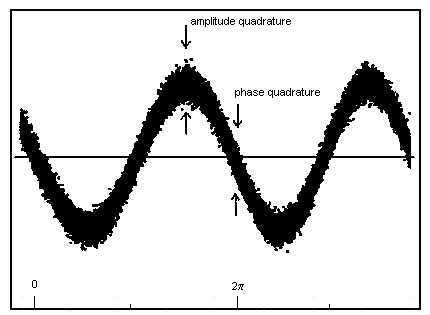Shown below is the measurement of the quantum noise of a coherent state's electrical field in dependance of its phase angle (= time). It is a sine wave broadened by the amount of its quantum noise.
  

The amount of a coherent state's quantum noise is not only independent of the wave's phase, but also of its amplitude. Thus with increasing amplitude the overall amount of quantum noise remains the same. However the relative signal to noise ratio (regarding the light wave itself as the signal) becomes better. This is one of the reasons why quantum effects of the light field become more or less unobservable for classical light waves, that is waves with large amplitudes. For such waves the influence of the very small amount of quantum noise is negligible in most cases. Shown below are the measurements of three laser waves with increasing amplitudes (notice the different scaling of the y-axis in units of the vacuum noise of the light field).

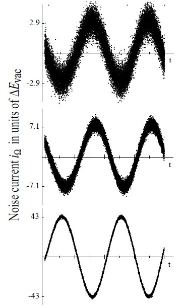
Notice that when the amplitude goes to zero the noise still remains there. This is the vacuum noise of the light's electrical field, corresponding to the mysterious 1/2 energy quantum that we met in the harmonic oscillator lessons in our first quantum mechanics classes. It corresponds to an intrinsic non-extractable field energy of a system without any excitation.
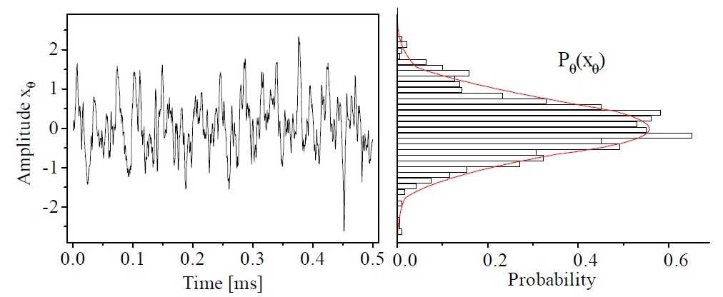
The probability distribution of the quantum noise at each phase angle is gained, by sampling the measured noise amplitude values. An example is shown in the next graph. The noise figure to the left represents a small section of one of the measurements shown above corresponding to a specific phase angle, the bins at the right form the corresponding field distribution function (rotated by 90°). In the case of a coherent state the resulting distribution can be fitted by a Gaussian (red line).

This probability distribution of the quantum noise at a certain time (= phase angle) corresponds to the state's wave packet, known from Schroedinger's description of quantum mechanics. Sampling the quantum noise at a whole series of time intervals, we obtain the wave packet at different times, thus we can observe the time evolution of the state's wave packet. The coherent state's wave packet oscillates evenly back and forth, similar to the movement of a classical particle within an harmonic potential. Unlike a classical particle however, there will be always a certain width of the wave packet, an uncertainty in its exact position. For a coherent state this width remains always the same throughout the whole oscillation period. This was the first example of quantum dynamics found by E. Schroedinger in 1926 (ref.1).  

Most instructively and compact the state of the light field is depicted by its Wigner function. This function was found by L. Szilard and E.P. Wigner some years before 1932 for "another purpose". The Wigner function is a phase space distribution similar to the Maxwell-Boltzmann distribution of position and momentum of an ensemble of particles known from classical statistical mechanics. It is not a probability distribution though, since due to the non-commutativity of position and momentum (i.e. phase- and amplitude-quadrature in the case of the light field) it may take on negative values. The wave packet is the density projection of the Wigner function distribution under various phase angles. Thus, measuring the wave packets probability distribution for a set of phase angles between 0 and pi as shown above, corresponds figuratively speaking to looking at the (non-measurable) Wigner function from different directions. The Wigner function can be gained from these experimental noise measurements via tomographical reconstruction techniques, inverse transformations similar to the ones applied in medical imaging (ref.3,4). First measurements of this kind were done in the group of Prof. Raymer in Oregon (ref.9).
Looking at the illustration below you see that you can regard Schroedinger's wave packet either as a glimpse at the unmeasurable Wigner function at a specific moment, or as the statistical distribution of a series of measurements of the quantum object (the light wave) at a specific time interval (phase angle).

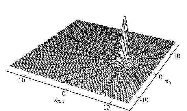
The coherent state's Wigner function is rotationally symmetric, due to the phase-independence of its quantum noise. It is displaced from the origin by the amount of the state's amplitude. Shown below is the Wigner function gained from the measured wave packet distributions shown above. (x and y or x0 and xp/2 denote the phase and amplitude quadrature)