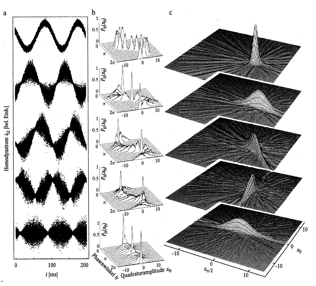
A splendid demonstration of Heisenberg's uncertainty principle can be given by reducing the quantum noise in one quadrature of the light field (for example the phase) on the expense of enhancing it in the complementary observable (i.e. the amplitude, or vice versa). This can be done by methods of nonlinear optics, for example parametric amplification and deamplification (see chap. 4). The so generated states of the light field are called squeezed states since the quantum noise got squeezed at a specific phase angle. Their wave packets do not only move back and forth in time like the ones you have seen for the coherent state, they also get wider and narrower: they breathe. The corresponding phase space distribution has an elliptical shape. Squeezed states have been investigated in many experiments in the past 15 years (refs.6-11,19-23), since they can be used to reduce the amount of noise in specially designed optical precision measurements. The amount of squeezing, the amplitude of the coherent excitation as well as the relative angle between the squeezed quadrature and the coherent excitation of the light can vary. Thus there is a whole family of such squeezed states of light. The following graphs show the measured quantum noise (a), moving wave packets (b) and Wigner functions (c) of characteristic representatives of this family. The degree of squeezing, i.e. the amount of noise reduction is a factor of four in the squeezed quadrature for the presented measurements. The shifting of the squeezing angle corresponds to a rotation of the state's distribution in phase space. From the top: coherent state, phase-squeezed state, 48°-squeezed state, amplitude-squeezed state, squeezed-vacuum state.
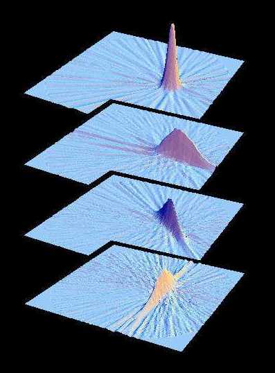
In color:
Knowing the evolution of the wave packet or the Wigner function, we can
readily deduce the distribution of
energy quanta, the photons, that build up the light
wave (see refs.4,17). On the other hand, knowing the distribution of photons does not
necessarily allow us to indicate the state of the light field, since they contain no information about the state's phase.
See in the next chapter
some examples of states which possess the same photon number distribution but completely
different Wigner functions and wave packets. The photon number distribution is given by
the diagonal elements of another complete description of the state of the light
field: the
density matrix .
in the
Fock (number state) representation
which we will denote by (ρnm).
The diagonal elements of the
density matrix contain the information about the intensity distribution of the state, the
phase information is hidden in the off-diagonal elements. Mathematically the density
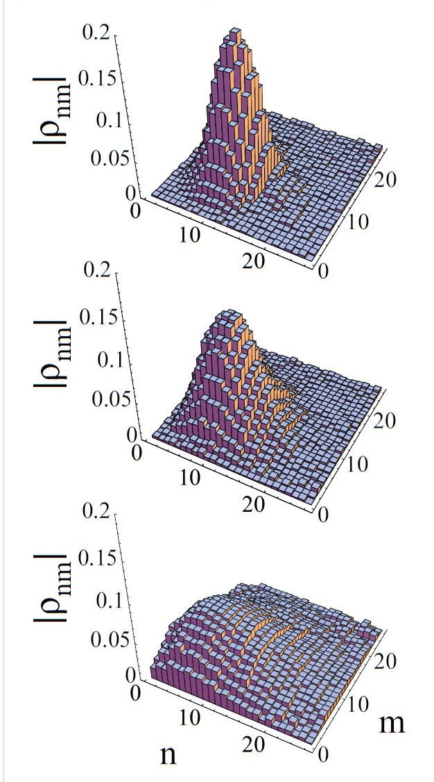
matrix is perfectly equivalent to the phase space distribution shown before. See below the
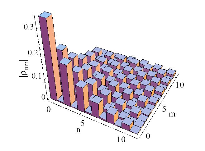
measured density matrices of (from top to bottom) an amplitude-squeezed, a coherent and a phase-squeezed state.
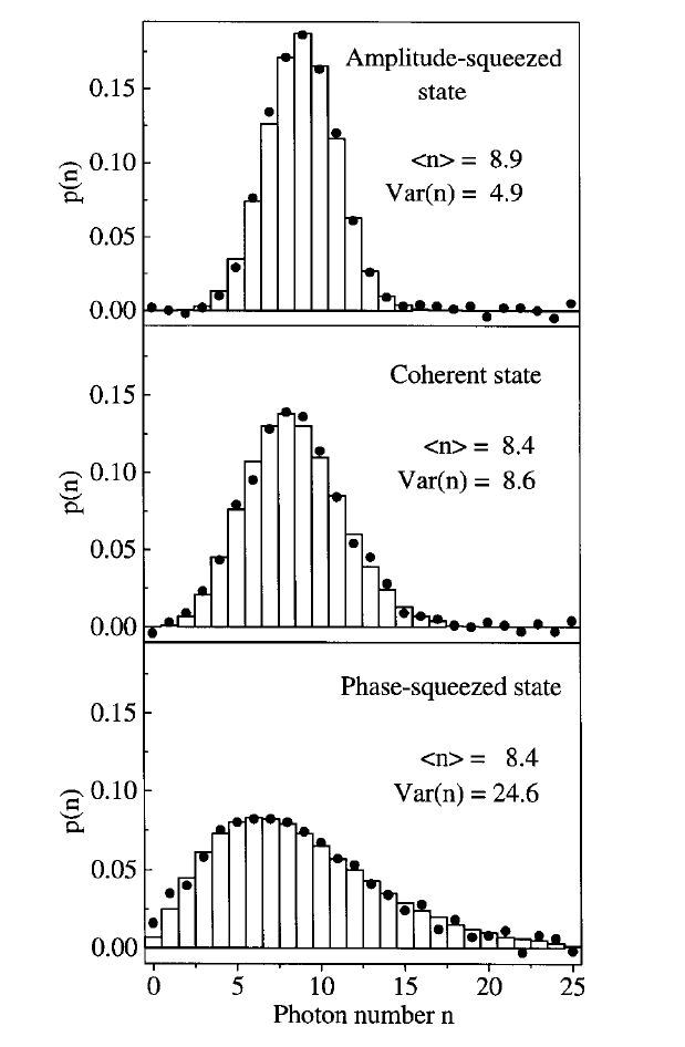
Analyzing the diagonal elements of the three matrices shown above we find, that the photon number distribution of the coherent state is Poissonian, thus the mean photon number <n> is equal to the spreading of the photon number distribution, its variance Var(n). For the other states we find roughly the more enhanced the state's amplitude noise, the more spread out is its photon number distribution i.e. the more enhanced its intensity noise. Thus, for the amplitude-squeezed state the photon number variance is less than the mean photon number. Such light is called sub-Poissonian light. It has played an important role in the history of quantum optics, since it was the first kind of non-classical light that has been detected. Note however that not all amplitude-squeezed light is sub-Poissonian (for example states with a very small amplitude, see refs 11,12), and vice versa sub-Poissonian light may very well be not amplitude-squeezed, for example if it is classically not coherent, phase diffused. The phase-squeezed light on the other hand has a much broader super-Poissonian photon number distribution than the coherent state.
(bars - theory, dots - experimental values)
The experimental significance of these distributions is the following: When we measure
the light field with photon counters, that is detectors that produce a single electrical "click" whenever it
is hit by a single photon, then the height of the bar in the graph above tells us how likely it will be that the
detector is hit by n photons at the same time (or more precisely within the same time interval defined
by the detectors response). This will be more clear when looking at the next example.
A most interesting structure is found for the density matrix of the
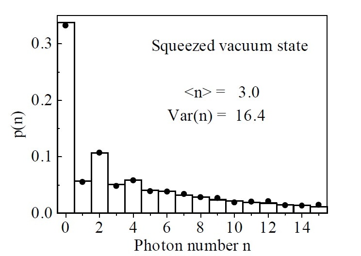
squeezed vacuum state: Due to its phase space symmetry the matrix displays a chessboard
pattern.
Analyzing the diagonal elements of this density matrix we find that the photon number distribution exhibits odd-even oscillations. These can be explained by quantum interference in phase space (ref 5), or equivalently by the nonlinear generation process of the state (see chapter 4): One photon of high energy is split into two photons, each containing half the energy of the original pump photon. Thus it is more likely that the detector will be hit by pairs of photons than by single ones. Note also that the squeezed vacuum in contrast to a vacuum state does have a non-vanishing mean photon number. The state is always strongly super-Poissonian.
A very curious role falls to the off-diagonal elements share: As it has been said above, they hide
the phase information. In direct interpretation though, their magnitude represents the transition probabilities
for the state to change its photon number from n to m. So for a light wave to be coherent it is
by all means necessary (though by no means sufficient) to have a constantly varying photon number.
This becomes more obvious when looking at the states' phase distribution.
The phase distribution is another non-complete representation of the
quantum state, complementary to the photon number distribution. Figuratively you
can think of the phase operator as being a light house situated at its port, the
origin of the phase space, throwing light on the physe space distributions around it. Thus the
phase distribution of a coherent state will be the narrower the more distant the state is
situated from the origin, i.e. the larger its amplitude. Therefore when comparing
phase distributions of different kinds of states, the states should have the same
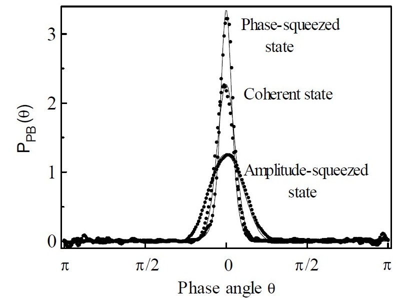
amplitude. A measurement (reconstructed via the density matrix) of the three
differently squeezed states of roughly the same amplitude presented above is shown
in the next graph. As expected, the phase distribution of the phase-squeezed state is
a lot narrower than that of the coherent state and the broadest distribution belongs to the
amplitude-squeezed state.
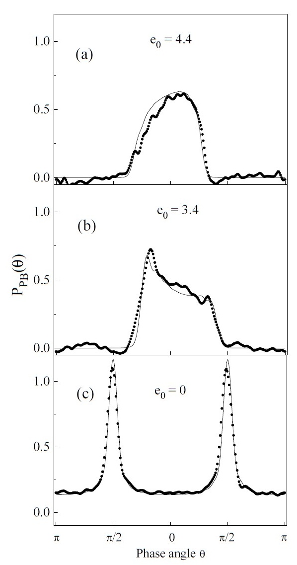
When the amplitude-squeezed state gets shifted closer and closer to the phase space origin by reducing its amplitude e0 (average photon number n = e0/2 ) its phase distribution broadens more and more and then suddenly exhibits a bifurcation: it splits into two peaks. Figuratively this can be understood using the light house picture again: The more the state approaches the origin, the more particular features, for example rotational asymmetries, can be resolved by the phase operator. The figures below strikingly demonstrate this astonishing behaviour near the origin by measured data.
![]()